Trying to extract a hierarchical trace for smart data aggregation
Table of Contents
Sitemap
|
|


Jean-Marc, Robin and Lucas have this nice technique to aggregate data and depict such information using for example treemaps. Lucas was visiting us this week and some of the reviewers of one of their article asked for large non-synthetic traces. G5K has a natural hierarchy so we decided to try extract interesting information. Fortunately, Elodie, Pierre, and Bruno who are in the office next door and administrate G5K and Ciment could help and point us quickly to the right places. :)
Useful links
- https://intranet.grid5000.fr/ganglia/?p=2&c=Bordeaux&h=bordeplage-1.bordeaux.grid5000.fr
- https://www.grid5000.fr/mediawiki/index.php/API_all_in_one_Practical#Using_Restfully_as_a_shell
- https://www.grid5000.fr/mediawiki/index.php/API_Metrology_Practical
- https://www.grid5000.fr/gridstatus/oargridgantt.cgi?year=2012&month=Jul&day=10&hour=06:00&range=month&plus.x=23&plus.y=18
- https://helpdesk.grid5000.fr/oar/Nancy/drawgantt.cgi
- https://intranet.grid5000.fr/oar/grenoble/digitalis/
- https://intranet.grid5000.fr/supervision/grenoble/weathermap/
Obtain useful information via REST
sudo gem install restfully
restfully -u alegrand -p 'myg5kpassword' --uri https://api.grid5000.fr/stable/grid5000
Here is a first attempt to obtain the machine load. The good thing with interactive ruby and object inspection is you can simply tab to obtain the list of methods and explore the object:
# I could browse like this:
root.sites[:rennes].clusters[:parapide].nodes[:'parapide-1'] # this allows to iterate per site/cluster/node but provides mainly static informations
# To access ganglia information, you have to look at the metrics field:
pp root.sites[:rennes].metrics[:cpu_idle].timeseries[:'paradent-5']
# It is even possible to filter a bit
pp root.sites[:rennes].metrics[:cpu_idle].timeseries.load(:query => {:resolution => 15, :from => Time.now.to_i-3600*1})[:'paradent-5']
# So for a particular node, the last measured value is:
root.sites[:rennes].metrics[:cpu_idle].timeseries[:'paradent-5'].properties['values'][0]

# So let's iterate over all machines
file = File.open("/tmp/rest.txt", 'w')
root.sites.each do |site|
  site.metrics[:cpu_idle].timeseries.each do |node|
    file.write node.properties['hostname'] + ", " + node.properties['values'][0].to_s + "\n"
  end
end
file.close
Unfortunately, this provides a rather poor information as only running nodes that are not deployed may return this information:
tail /tmp/rest.txt
pastel-62.toulouse.grid5000.fr,
pastel-83.toulouse.grid5000.fr,
pastel-63.toulouse.grid5000.fr,
pastel-55.toulouse.grid5000.fr,
pastel-56.toulouse.grid5000.fr, 99.9
pastel-140.toulouse.grid5000.fr,
pastel-76.toulouse.grid5000.fr, 100.0
pastel-57.toulouse.grid5000.fr, 100.0
pastel-21.toulouse.grid5000.fr, 99.875
pastel-77.toulouse.grid5000.fr,
grep ', [0-9]' /tmp/res.txt | wc -l
cat /tmp/res.txt | wc -l
622
1426
So instead, let's try to capture the state of the machines:
file = File.open("/tmp/state_rest.txt", 'w')
root.sites.each do |site|
  site.status.each do |node|
    file.write site.properties['uid'] + "/" + node.properties['node_uid'] + ", " + node.properties['system_state'] + "\n"
  end
end
file.close
tail /tmp/state_rest.txt
toulouse/pastel-6, unknown
toulouse/pastel-93, free
toulouse/pastel-37, unknown
toulouse/pastel-65, unknown
toulouse/pastel-7, unknown
toulouse/pastel-94, unknown
toulouse/pastel-38, free
toulouse/pastel-114, free
toulouse/pastel-66, free
toulouse/pastel-8, besteffort
sed 's/.*, //' /tmp/state_rest.txt | sort | uniq
for i in `sed 's/.*, //' /tmp/state_rest.txt | sort | uniq` ; do echo "$i :" `grep $i /tmp/state_rest.txt | wc -l` ; done
besteffort : 150
busy : 232
free : 582
unknown : 205
So we could set up an observation for a month but this would be long. Instead we decided we should rather try to get all this information from the OAR database.
Useful information from OAR mysql
Dumping the database
I wanted to first get a local version to browse it more comfortably.
ssh access.grenoble.grid5000.fr "mysqldump --lock-tables=false --quick -uoarreader -pread -h mysql.grenoble.grid5000.fr oar2" > oar2.sql
cat oar2.sql | mysql -u root -p$PASSWORD -h localhost oar2-grenoble
Obviously, when we will work on getting such information for all sites, we should dump to csv remotely to save space.
Looking at the tables, here is what I found that may be of interest for us:
- resources:
- resource_id
- network_address
- cpu
- cpuset
- jobs
- job_id
- start_time
- stop_time
- assigned_resources
- moldable_job_id
- resource_id
- resource_logs
- resource_id
- date_start
- attribute
- value
- job_types
- job_id
- type
OK, so let's write a tiny script to extract the right information:
echo $FIELDS > /tmp/$TABLE.csv
echo "SELECT $FIELDS FROM $TABLE INTO OUTFILE \"/tmp/foo.csv\" FIELDS TERMINATED BY ',' ENCLOSED BY '\"' LINES TERMINATED BY \"\\n\"" | mysql -u root -p$PASSWORD -h localhost $DATABASE
cat /tmp/foo.csv >> /tmp/$TABLE.csv
And let's call it for the different tables I am interested in (see in the org source at the bottom of the page how I reuse the previous block to do the job)…
Having fun with R
OK, now, I can read these information and exploit them in R.
jobs <- read.csv("/tmp/jobs.csv")
jobs <- jobs[jobs$start_time>3000,]             #cleanups
jobs <- jobs[jobs$stop_time>3000,]              #cleanups
jobs <- jobs[jobs$stop_time>jobs$start_time,]   #cleanups
assigned_resources <- read.csv("/tmp/assigned_resources.csv")
job_types <- read.csv("/tmp/job_types.csv")
resources <- read.csv("/tmp/resources.csv")
resource_logs <- read.csv("/tmp/resource_logs.csv")
names(resource_logs)=c("resource_id", "start_time", "attribute", "state")
resource_logs <- resource_logs[resource_logs$attribute=="state",]
resource_logs <- resource_logs[!(names(resource_logs) %in% c("attribute"))]
Let's select at random a week time interval.
start <- sample(jobs$start_time, 1)
end <- start+7*24*3600
job_resources <- merge(jobs[jobs$stop_time<=end & jobs$start_time>=start,],assigned_resources,by.x="job_id",by.y="moldable_job_id")
job_resources <- merge(job_resources,job_types,by.x="job_id",by.y="job_id")
job_resources <- merge(job_resources,resources,by.x="resource_id",by.y="resource_id")

# Mmmh, I need to get resource_state into a similar format so that dataframes can be merged
resource_states <- resource_logs[resource_logs$start_time <=end & resource_logs$start_time >= start, ]
resource_states <- resource_states[with(resource_states, order(resource_id,start_time)),]
block <- function(proc) {
  end_v <- c(tail(proc$start_time,length(proc$start_time)-1),end)
  cbind(proc,stop_time=end_v)
}
compute_durations <- function(df) {
  d <- data.frame()
  for(rank in unique(df$resource_id)) {
    d=rbind(d,block(df[df$resource_id==rank,]))
  }
  d
}
resource_states <- compute_durations(resource_states)
resource_states <- resource_states[resource_states$state != "Alive",]
resource_states <- merge(resource_states,resources,by.x="resource_id",by.y="resource_id")
names(resource_states)[names(resource_states)%in% c("state")] <- "type"
df <- rbind.fill(resource_states,job_resources)
And voilà, I can plot the Gantt chart now.
library(ggplot2)
ggplot(df)+
    theme_bw()+geom_rect(aes(xmin=start_time,xmax=stop_time, ymin=resource_id, ymax=resource_id+1,fill=factor(type)))
# + scale_y_continuous(limits=c(min(as.numeric(df_native$ResourceId)),max(as.numeric(df_native$ResourceId))+1))
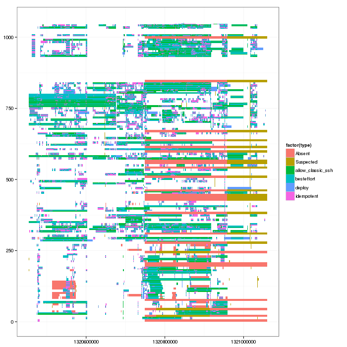
So now Lucas can convert such thing into a simple Paje trace and use triva to see whether he can turn this into interesting visualizations.
Entered on